I read a great deal of technical literature and highly recommend the same for anyone interested in developing their skill in this field. While many recent publications have proven worthwhile (2011's update of Data Mining by Witten and Frank; and 2010's Fundamentals of Predictive Text Mining, by Weiss, Indurkhya and Zhang are good examples), I confess being less than overwhelmed by many current offerings in the literature. I will not name names, but the first ten entries returned from my search of books at Amazon for "big data" left me unimpressed. While this field has enjoyed popular attention because of a colorful succession of new labels ("big data" merely being the most recent), many current books and articles remain too far down the wrong end of the flash/substance continuum.
For some time, I have been exploring older material, some from as far back as the 1920s. A good example would be a certain group of texts I've discovered, from the 1950s and 1960s- a period during which the practical value of statistical analysis had been firmly established in many fields, but long before the arrival of cheap computing machinery. At the time, techniques which maximized the statistician's productivity were ones which were most economical in their use of arithmetic calculations.
I first encountered such techniques in Introduction to Statistical Analysis, by Dixon and Massey (my edition is from 1957). Two chapters, in particular, are pertinent: "Microstatistics" and "Macrostatistics", which deal with very small and very large data sets, respectively (using the definitions of that time). One set of techniques described in this book involve the calculation of the mean and standard deviation of a set of numbers from a very small subset of their values. For instance, the mean of just 5 values- percentiles 10, 30, 50, 70 and 90- estimates the mean with 93% statistical efficiency.
How is this relevant to today's analysis? Assuming that the data is already sorted (which it often is, for tree induction techniques), extremely large data sets can be summarized with a very small number of operations (4 additions and 1 division, in this case), without appreciably degrading the quality of the estimate.
Data storage has grown faster than computer processing speed. Today, truly vast collections of data are easily acquired by even tiny organizations. Dealing with such data requires finding methods to accelerate information processing, which is exactly what authors in the 1950s and 1960s were writing about.
Readers may find a book on exactly this subject, Nonparametric and Shortcut Statistics, by Tate and Clelland (my copy is from 1959), to be of interest.
Quite a bit was written during the time period in question regarding statistical techniques which: 1. made economical use of calculation, 2. avoided many of the usual assumptions attached to more popular techniques (normal distributions, etc.) or 3. provided some resistance to outliers.
Genuinely new ideas, naturally, continue to emerge, but don't kid yourself: Much of what is standard practice today was established years ago. There's a book on my shelf, Probabilistic Models, by Springer, Herlihy, Mall and Beggs, published in 1968, which describes in detail what we would today call a naive Bayes regression model. (Indeed, Thomas Bayes' contributions were published in the 1760s.) Claude Shannon described information and entropy- today commonly used in rule- and tree-induction algorithms as well as regression regularization techniques- in the late 1940s. Logistic regression (today's tool of choice in credit scoring and many medical analyses) was initially developed by Pearl and Reed in the 1920s, and the logistic curve itself was used to forecast proportions (not probabilities) after being introduced by Verhulst in the late 1830s.
Ignore the history of our field at your peril.
Showing posts with label Shannon. Show all posts
Showing posts with label Shannon. Show all posts
Saturday, November 23, 2013
Sunday, September 12, 2010
Reader Question: Putting Entropy to Work
Introduction
In response to my Nov-10-2006 posting, Introduction To Entropy, an anonymous reader asked:
Can we use entropy for distinguishing random signals and deterministic signal? Lets say i generate two signals in matlab. First signal using sin function and second using randn function. Can we use entropy to distinguish between these two signal?
The short answer is: Yes, we can use entropy for this purpose, although even simpler summary statistics would reveal that the normally distributed randn data included values outside of -1..+1, while the sin data did not.
In this article, I will be using my own entropy calculating routines, which can be found on MATLAB Central: Entropy, JointEntropy, ConditionalEntropy and MutualInformation.
A Slightly Harder Problem
To illustrate this application of entropy, I propose a slightly different problem, in which the sine data and the random data share the same distribution. To achieve this, the "random" data will be a random sample from the sine function:
>> X = [1:1000]';
>> Sine = sin(0.05 * X);
>> RandomData = sin(2 * pi * rand(size(X)));
As a quick check on the distributions, we will examine their respective histograms:
>> figure
>> subplot(2,1,1), hist(Sine), xlabel('Sine Value'), ylabel('Frequency'), grid on
>> subplot(2,1,2), hist(RandomData), xlabel('RandomData Value'), ylabel('Frequency'), grid on

Click image to enlarge.
More or less, they appear to match.
A First Look, Using Entropy
At this point, the reader may be tempted to calculate the entropies of the two distributions, and compare them. Since their distributions (as per the histograms) are similar, we should expect their entropies to also be similar.
To date, this Web log has only dealt with discrete entropy, yet our data is continuous. While there is a continuous entropy, we will stick with the simpler (in my opinion) discrete entropy for now. This requires that the real-valued numbers of our data be converted to symbols. We will accomplish this via quantization ("binning") to 10 levels:
>> Sine10 = ceil(10 * (Sine + 1) / 2);
>> RandomData10 = ceil(10 * (RandomData + 1) / 2);
If the MATLAB Statistics Toolbox is installed, one can check the resulting frequencies thus (I apologize for Blogger's butchering of the text formatting):
>> tabulate(Sine10)
Value Count Percent
1 205 20.50%
2 91 9.10%
3 75 7.50%
4 66 6.60%
5 60 6.00%
6 66 6.60%
7 66 6.60%
8 75 7.50%
9 91 9.10%
10 205 20.50%
>> tabulate(RandomData10)
Value Count Percent
1 197 19.70%
2 99 9.90%
3 84 8.40%
4 68 6.80%
5 66 6.60%
6 55 5.50%
7 68 6.80%
8 67 6.70%
9 82 8.20%
10 214 21.40%
It should be noted that other procedures could have been used for the signal-to-symbol conversion. For example, bin frequencies could have been made equal. The above method was selected because it is simple and requires no Toolbox functions. Also, other numbers of bins could have been utilized.
Now that the data is represented by symbols, we may check the earlier assertion regarding similar distributions yielding similar entropies (measured in bits per observation):
>> Entropy(Sine10)
ans =
3.1473
>> Entropy(RandomData10)
ans =
3.1418
As these are sample statistics, we would not expect them to match exactly, but these are very close.
Another Perspective
One important aspect of the structure of a sine curve is that it varies over time (or whatever the domain is). This means that any given sine value is typically very similar to those on either side. With this in mind, we will investigate the conditional entropy of each of these two signals versus themselves, lagged by one observation:
>> ConditionalEntropy(Sine10(2:end),Sine10(1:end-1))
ans =
0.6631
>> ConditionalEntropy(RandomData10(2:end),RandomData10(1:end-1))
ans =
3.0519
Ah! Notice that the entropy of the sine data, given knowledge of its immediate predecessor is much lower than the entropy of the random data, given its immediate predecessor. These data are indeed demonstrably different insofar as they behave over time, despite sharing the same distribution.
An astute reader may at this point notice that the conditional entropy of the random data, given 1 lagged value, is less than the entropy of the raw random data. This is an artifact of the finite number of samples and the quantization process. Given more observations and a finer quantization, this discrepancy between sample statistics and population statistics will shrink.
Entropy could have been applied to this problem other ways, too. For instance, one might calculate entropy for short time windows. I would point out that other, more traditional procedures might be used instead, such as calculating the auto-correlation for lag 1. It is worth seeing how entropy adds to the analyst's toolbox, though.
Further Reading
See also the Apr-01-2009 posting, Introduction to Conditional Entropy.
Print:
The Mathematical Theory of Communication by Claude Shannon (ISBN 0-252-72548-4)
Elements of Information Theory by Cover and Thomas (ISBN 0-471-06259)
Wednesday, April 01, 2009
Introduction to Conditional Entropy
Introduction
In one of the earliest posts to this log, Introduction To Entropy (Nov-10-2006), I described the entropy of discrete variables. Finally, in this posting, I have gotten around to continuing this line of inquiry and will explain conditional entropy.
Quick Review: Entropy
Recall that entropy is a measure of uncertainty about the state of a variable. In the case of a variable which can take on only two values (male/female, profit/loss, heads/tails, alive/dead, etc.), entropy assumes its maximum value, 1 bit, when the probability of the outcomes is equal. A fair coin toss is a high-entropy event: Beforehand, we have no idea about what will happen. As the probability distribution moves away from a 50/50 split, uncertainty about the outcome decreases since there is less uncertainty as to the outcome. Recall, too, that entropy decreases regardless of which outcome class becomes the more probable: an unfair coin toss, with a heads / tails probability distribution of 0.10 / 0.90 has exactly the same entropy as another unfair coin with a distribution of 0.90 / 0.10. It is the distribution of probabilities, not their order which matters when calculating entropy.
Extending these ideas to variables with more than 2 possible values, we note that generally, distributions which are evenly spread among the possible values exhibit higher entropy, and those which are more concentrated in a subset of the possible values exhibit lower entropy.
Conditional Entropy
Entropy, in itself, is a useful measure of the mixture of values in variables, but we are often interested in characterizing variables after they have been conditioned ("modeled"). Conditional entropy does exactly that, by measuring the entropy remaining in a variable, after it has been conditioned by another variable. I find it helpful to think of conditional entropy as "residual entropy". Happily for you, I have already assembled a MATLAB function, ConditionalEntropy, to calculate this measure.
As an example, think of sporting events involving pairs of competitors, such as soccer ("football" if you live outside of North America). Knowing nothing about a particular pair of teams (and assuming no ties), the best probability we may assess that any specific team, say, the Black Eagles (Go, Beşiktaş!), will win is:
p(the Black Eagles win) = 0.5
The entropy of this variable is 1 bit- the maximum uncertainty possible for a two-category variable. We will attempt to lower this uncertainty (hence, lowering its conditional entropy).
In some competitive team sports, it has been demonstrated statistically that home teams have an advantage over away teams. Among the most popular sports, the home advantage appears to be largest for soccer. One estimate shows that (excluding ties) home teams have historically won 69% of the time, and away teams 31% of the time. Conditioning the outcome on home vs. away, we may provide the follwing improved probability estimates:
p(the Black Eagles win, given that they are the home team) = 0.69
p(the Black Eagles win, given that they are the away team) = 0.31
Ah, Now there is somewhat less uncertainty! The entropy for probability 0.69 is 0.8932 bits. The entropy for probability 0.31 (being the same distance from 0.5 as 0.69) is also 0.8932 bits.
Conditional entropy is calculated as the weighted average of the entropies of the various possible conditions (in this case home or away). Assuming that it is equally likely that the Black Eagles play home or away, the conditional entropy of them winning is 0.8932 bits = (0.5 * 0.8932 + 0.5 * 0.8932). As entropy has gone down with our simple model, from 1 bit to 0.8932 bits, we learn that knowing whether the Black Eagles are playing at home or away provides information and reduces uncertainty.
Other variables might be used to condition the outcome of a match, such as number of player injuries, outcome of recent games, etc. We can compare these candidate predictors using conditional entropy. The lower the conditional entropy, the lower the remaining uncertainty. It is even possible to assess a combination of predictors by treating each combination of univariate conditions as a separate condition ("symbol", in information theoretic parlance), thus:
p(the Black Eagles win, given:
that they are the home team and there are no injuries) = ...
that they are the away team and there are no injuries) = ...
that they are the home team and there is 1 injury) = ...
that they are the away team and there is 1 injury) = ...
etc.
My routine, ConditionalEntropy can accommodate multiple conditioning variables.
Conclusion
The models being developed here are tables which simplistically cross all values of all input variables, but conditional entropy can also, for instance, be used to evaluate candidate splits in decision tree induction, or to assess class separation in discriminant analysis.
Note that, as the entropies calculated in this article are based on sample probabilities, they suffer from the same limitations as all sample statistics (as opposed to population statistics). A sample entropy calculated from a small number observations likely will not agree exactly with the population entropy.
Further Reading
See also my Sep-12-2010 posting, Reader Question: Putting Entropy to Work.
Print:
The Mathematical Theory of Communication by Claude Shannon (ISBN 0-252-72548-4)
Elements of Information Theory by Cover and Thomas (ISBN 0-471-06259)
Friday, November 10, 2006
Introduction To Entropy
The two most common general types of abstract data are numeric data and class data. Basic summaries of numeric data, like the mean and standard deviation are so common that they have even been encapsulated as functions in spreadsheet software.
Class (or categorical) data is also very common. Class data has a finite number of possible values, and those values are unordered. Blood type, ZIP code, ice cream flavor and marital status are good examples of class variables. Importantly, note that even though ZIP codes, for instance, are "numbers", the magnitude of those numbers is not meaningful.
For the purposes of this article, I'll assume that classes are coded as integers (1 = class 1, 2 = class 2, etc.), and that the numeric order of these codes are meaningless.
How can class data be summarized? One very simple class summary is a list of distinct values, which MATLAB provides via the unique function. Slightly more complex is the frequency table (distinct values and their counts), which can be generated using the tabulate function from the Statistics Toolbox, or one's own code in base MATLAB, using unique:
>> MyData = [1 3 2 1 2 1 1 3 1 1 2]';
>> UniqueMyData = unique(MyData)
UniqueMyData =
1
2
3
>> nUniqueMyData = length(UniqueMyData)
nUniqueMyData =
3
>> FreqMyData = zeros(nUniqueMyData,1);
>> for i = 1:nUniqueMyData, FreqMyData(i) = sum(double(MyData == UniqueMyData(i))); end
>> FreqMyData
FreqMyData =
6
3
2
The closest thing to an "average" for class variables is the mode, which is the value (or values) appearing most frequently and can be extracted from the frequency table.
A number of measures have been devised to assess the "amount of mix" found in class variables. One of the most important such measures is entropy. This would be roughly equivalent to "spread" in a numeric variable.
I will define entropy for two-valued variables, but it is worth first conducting a thought experiment to understand how such a measure should work. Consider a variable which assumes only 2 values, like a coin toss. The outcome of a series of coin tosses is a variable which can be characterized by its probability of coming up "heads". If the probability is 0.0 ("tails" every time) or 1.0 (always "heads"), then there isn't any mix of values at all. The maximum mix will occur when the probability of "heads" is 0.5- a fair coin toss. Let's assume that our measure of mixture varies on a scale from 0.0 ("no mix") to 1.0 ("maximum mix"). This means that our measurement function would yield a 0.0 at a probability of 0.0 (pure tails), rise to 1.0 at a probability of 0.5 (maximum impurity), and fall back to 0.0 at a probability of 1.0 (pure heads).
Entropy is exactly such a measure. It was devised in the late 1940s by Claude Shannon when he invented information theory (then known as communication theory). Entropy can be applied to variables with more than two values, but graphing the two-value case is much more intuitive (click the graph to enlarge):
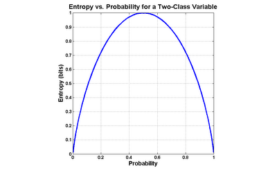
The formula for entropy in the case of a two-valued variable is as follows:
entropy = -( p * log(p) + (1-p) * log(1-p) )
...where p is the probability of one class (it doesn't matter which one).
Most often, base 2 logarithms are used, which means that the calculated entropy is in units of bits. Generally, the more distinct values in the variable, and the more evenly they are distributed, the greater the entropy. As an example, variables with completely even distributions of values possess 1 bit of entropy when there are 2 values, 2 bits when there are 4 values and 3 bits when there are 8 values. The less evenly those values are distributed, the lower the entropy. For instance, a 4-valued variable with a 40%/20%/20%/20% split has an entropy of 1.92 bits.
Entropy is frequently used in machine learning and data mining algorithms for things like feature selection or evaluating splits in decision trees.
I have written a MATLAB routine to calculate the entropy of sample data in MATLAB (see details in help Entropy):
Entropy
This routine calculates the entropy of each column in the provided matrix, and will handle more than 2 distinct values per variable.
Further Reading / References
See, also, my postings of Apr-01-2009, Introduction to Conditional Entropy, and of Sep-12-2010, Reader Question: Putting Entropy to Work.
Note that, for whatever historical reason, entropy is typically labeled H in formulas, i.e.: H(X) means "entropy of X".
Print:
The Mathematical Theory of Communication by Claude Shannon (ISBN 0-252-72548-4)
Elements of Information Theory by Cover and Thomas (ISBN 0-471-06259)
On-Line:
Information Theory lecture notes (PowerPoint), by Robert A. Soni
course slides (PDF), by Rob Malouf
Information Gain tutorial (PDF), by Andrew Moore
Class (or categorical) data is also very common. Class data has a finite number of possible values, and those values are unordered. Blood type, ZIP code, ice cream flavor and marital status are good examples of class variables. Importantly, note that even though ZIP codes, for instance, are "numbers", the magnitude of those numbers is not meaningful.
For the purposes of this article, I'll assume that classes are coded as integers (1 = class 1, 2 = class 2, etc.), and that the numeric order of these codes are meaningless.
How can class data be summarized? One very simple class summary is a list of distinct values, which MATLAB provides via the unique function. Slightly more complex is the frequency table (distinct values and their counts), which can be generated using the tabulate function from the Statistics Toolbox, or one's own code in base MATLAB, using unique:
>> MyData = [1 3 2 1 2 1 1 3 1 1 2]';
>> UniqueMyData = unique(MyData)
UniqueMyData =
1
2
3
>> nUniqueMyData = length(UniqueMyData)
nUniqueMyData =
3
>> FreqMyData = zeros(nUniqueMyData,1);
>> for i = 1:nUniqueMyData, FreqMyData(i) = sum(double(MyData == UniqueMyData(i))); end
>> FreqMyData
FreqMyData =
6
3
2
The closest thing to an "average" for class variables is the mode, which is the value (or values) appearing most frequently and can be extracted from the frequency table.
A number of measures have been devised to assess the "amount of mix" found in class variables. One of the most important such measures is entropy. This would be roughly equivalent to "spread" in a numeric variable.
I will define entropy for two-valued variables, but it is worth first conducting a thought experiment to understand how such a measure should work. Consider a variable which assumes only 2 values, like a coin toss. The outcome of a series of coin tosses is a variable which can be characterized by its probability of coming up "heads". If the probability is 0.0 ("tails" every time) or 1.0 (always "heads"), then there isn't any mix of values at all. The maximum mix will occur when the probability of "heads" is 0.5- a fair coin toss. Let's assume that our measure of mixture varies on a scale from 0.0 ("no mix") to 1.0 ("maximum mix"). This means that our measurement function would yield a 0.0 at a probability of 0.0 (pure tails), rise to 1.0 at a probability of 0.5 (maximum impurity), and fall back to 0.0 at a probability of 1.0 (pure heads).
Entropy is exactly such a measure. It was devised in the late 1940s by Claude Shannon when he invented information theory (then known as communication theory). Entropy can be applied to variables with more than two values, but graphing the two-value case is much more intuitive (click the graph to enlarge):
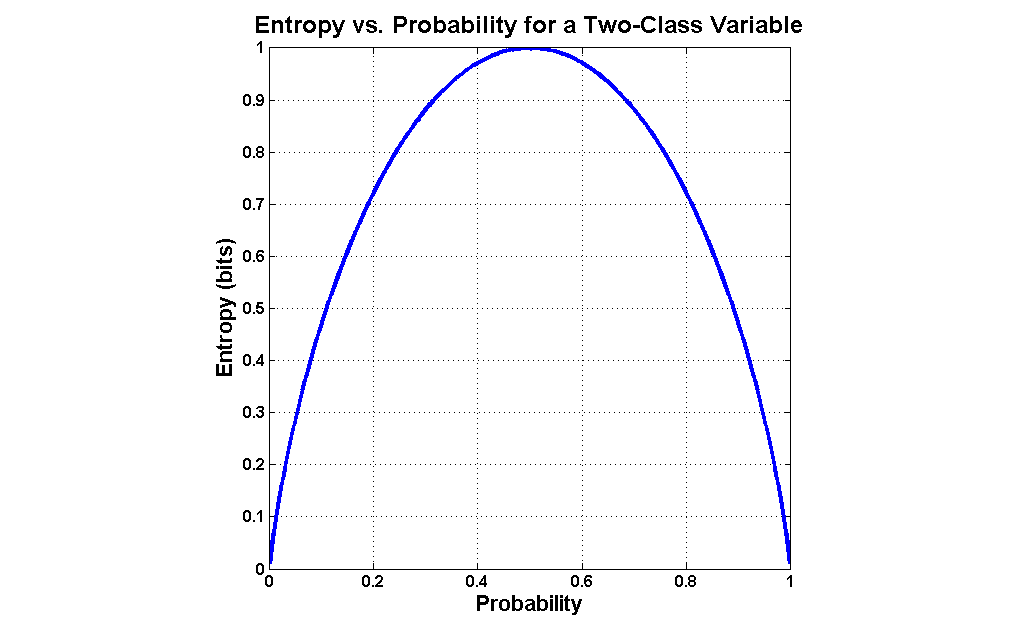
The formula for entropy in the case of a two-valued variable is as follows:
entropy = -( p * log(p) + (1-p) * log(1-p) )
...where p is the probability of one class (it doesn't matter which one).
Most often, base 2 logarithms are used, which means that the calculated entropy is in units of bits. Generally, the more distinct values in the variable, and the more evenly they are distributed, the greater the entropy. As an example, variables with completely even distributions of values possess 1 bit of entropy when there are 2 values, 2 bits when there are 4 values and 3 bits when there are 8 values. The less evenly those values are distributed, the lower the entropy. For instance, a 4-valued variable with a 40%/20%/20%/20% split has an entropy of 1.92 bits.
Entropy is frequently used in machine learning and data mining algorithms for things like feature selection or evaluating splits in decision trees.
I have written a MATLAB routine to calculate the entropy of sample data in MATLAB (see details in help Entropy):
Entropy
This routine calculates the entropy of each column in the provided matrix, and will handle more than 2 distinct values per variable.
Further Reading / References
See, also, my postings of Apr-01-2009, Introduction to Conditional Entropy, and of Sep-12-2010, Reader Question: Putting Entropy to Work.
Note that, for whatever historical reason, entropy is typically labeled H in formulas, i.e.: H(X) means "entropy of X".
Print:
The Mathematical Theory of Communication by Claude Shannon (ISBN 0-252-72548-4)
Elements of Information Theory by Cover and Thomas (ISBN 0-471-06259)
On-Line:
Information Theory lecture notes (PowerPoint), by Robert A. Soni
course slides (PDF), by Rob Malouf
Information Gain tutorial (PDF), by Andrew Moore
Subscribe to:
Posts (Atom)