Friday, November 17, 2006

Mahalanobis Distance

Many data mining and pattern recognition tasks involve calculating abstract "distances" between items or collections of items. Some modeling algorithms, such as k-nearest neighbors or radial basis function neural networks, make direct use of multivariate distances. One very useful distance measure, the Mahalanobis distance, will be explained and implemented here.


Euclidean Distance

The Euclidean distance is the geometric distance we are all familiar with in 3 spatial dimensions. The Euclidean distance is simple to calculate: square the difference in each dimension (variable), and take the square root of the sum of these squared differences. In MATLAB:


% Euclidean distance between vectors 'A' and 'B', original recipe
EuclideanDistance = sqrt(sum( (A - B) .^ 2 ))


...or, for the more linear algebra-minded:


% Euclidean distance between vectors 'A' and 'B', linear algebra style
EuclideanDistance = norm(A - B)


This distance measure has a straightforward geometric interpretation, is easy to code and is fast to calculate, but it has two basic drawbacks:

First, the Euclidean distance is extremely sensitive to the scales of the variables involved. In geometric situations, all variables are measured in the same units of length. With other data, though, this is likely not the case. Modeling problems might deal with variables which have very different scales, such as age, height, weight, etc. The scales of these variables are not comparable.

Second, the Euclidean distance is blind to correlated variables. Consider a hypothetical data set containing 5 variables, where one variable is an exact duplicate of one of the others. The copied variable and its twin are thus completely correlated. Yet, Euclidean distance has no means of taking into account that the copy brings no new information, and will essentially weight the copied variable more heavily in its calculations than the other variables.


Mahalanobis Distance

The Mahalanobis distance takes into account the covariance among the variables in calculating distances. With this measure, the problems of scale and correlation inherent in the Euclidean distance are no longer an issue. To understand how this works, consider that, when using Euclidean distance, the set of points equidistant from a given location is a sphere. The Mahalanobis distance stretches this sphere to correct for the respective scales of the different variables, and to account for correlation among variables.

The mahal or pdist functions in the Statistics Toolbox can calculate the Mahalanobis distance. It is also very easy to calculate in base MATLAB. I must admit to some embarrassment at the simple-mindedness of my own implementation, once I reviewed what other programmers had crafted. See, for instance:

mahaldist.m by Peter J. Acklam

Note that it is common to calculate the square of the Mahalanobis distance. Taking the square root is generally a waste of computer time since it will not affect the order of the distances and any critical values or thresholds used to identify outliers can be squared instead, to save time.


Application

The Mahalanobis distance can be applied directly to modeling problems as a replacement for the Euclidean distance, as in radial basis function neural networks. Another important use of the Mahalanobis distance is the detection of outliers. Consider the data graphed in the following chart (click the graph to enlarge):


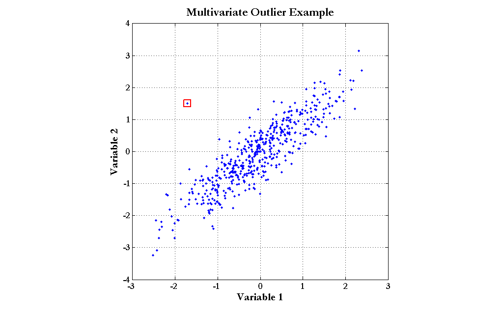
The point enclosed by the red square clearly does not obey the distribution exhibited by the rest of the data points. Notice, though, that simple univariate tests for outliers would fail to detect this point. Although the outlier does not sit at the center of either scale, there are quite a few points with more extreme values of both Variable 1 and Variable 2. The Mahalanobis distance, however, would easily find this outlier.


Further reading

Multivariate Statistical Methods, by Manly (ISBN: 0-412-28620-3)


Random MATLAB Link:

MATLAB array manipulation tips and tricks, by Peter J. Acklam


See Also

Mar-23-2007 posting, Two Bits of Code

Thursday, November 16, 2006

Fuzzy Logic In MATLAB Part 1

Fuzzy logic is a capable and often misunderstood analytical tool. A basic grasp of this technology may be gained from any of the following introductions to fuzzy logic:

Putting Fuzzy Logic to Work (PDF), PC AI magazine, by Dwinnell

Fuzzy Math, Part 1, The Theory, by Luka Crnkovic-Dodig

Fuzzy Logic Introduction (PDF), by Martin Hellmann

Fuzzy Logic Overview (HTML)

comp.ai.fuzzy FAQ: Fuzzy Logic and Fuzzy Expert Systems

Fuzzy Logic for "Just Plain Folks" (HTML), by Thomas Sowell


As a rule, in the interest of portability and transparency, I try to build as much of my code as possible in base MATLAB, and resort to using toolboxes and such only when neccessary. Fortunately, fuzzy logic is exceedingly easy to implement in the base MATLAB product.

Generation of fuzzy set memberships can be accomplished using the base MATLAB functions interp1 and pchip. Piecewise linear (most commonly: triangular and trapezoidal) fuzzy memberships can be calculated using the 'linear' method in interp1. Below is an example of a triangular fuzzy memebership function, defined over the Temperature domain (click the graph to enlarge):


The domain variable and shape parameters (domain vector followed by membership vector) control the form of the curve. Trapezoids are constructed by adding another element to each shape vector, like this:


Temperature = linspace(0,130,131);
Temp80ish = interp1([0 70 78 82 90 130],[0 0 1 1 0 0],Temperature,'linear');


Fuzzy membership functions with smoother transitions are possible by using the pchip function. The following depicts a bell-shaped membership function (as usual, click the graph to enlarge):


Of course, one is not limited to peaked or plateau-shaped fuzzy membership functions. The various interpolation and spline functions in MATLAB permit whatever irregular and arbitrary shapes may be called for.

In Part 2, I will build a small fuzzy rule base in MATLAB.


Further Reading

Print:

An excellent practical reference:
The Fuzzy Systems Handbook (Second Edition), by Cox (ISBN: 0121944557)

Tuesday, November 14, 2006

Finding MATLAB Source Code And Tools

Having read this log so far, you're probably pretty impressed, but thinking, "This is great stuff- really great stuff, but where else can I find MATLAB source code and tools for data mining?" There are four basic sources:

1. General Web Search Engines

Try searching for a combination of things:

Language:
MATLAB
"MATLAB source"
MATLAB AND "source code"

Algorithms:
backpropagation
"linear discriminant"
"neural network"

Some college professors give away high-quality material (papers and code) for free! This group of key phrases will help turn them up:

"course notes"
"course readings"
"lecture notes"
"syllabus"

Don't just use Google. I have found these search engines to be useful:


A9
AlltheWeb
Alta Vista
Devilfinder
Dogpile
Ixquick
Lycos


2. MATLAB Central

MATLAB Central


3. Source Code Repositories

Google Code
LiteratePrograms


4. Toolboxes

Commercial toolboxes are definitely the most expensive route to take, but there are free versions as well. This list is certainly not exhaustive.

The MathWorks

MATLAB Curve Fitting Toolbox
MATLAB Genetic Algorithm and Direct Search Toolbox
MATLAB Neural Network Toolbox
MATLAB Statistics Toolbox

Third-Party

glmlab (Generalized Linear Models in MATLAB)
The Lazy Learning Toolbox
MATLABArsenal
Netlab
PRTools
Statistical Pattern Recognition Toolbox
Stixbox
Support Vector Machine Toolbox

Friday, November 10, 2006

Introduction To Entropy

The two most common general types of abstract data are numeric data and class data. Basic summaries of numeric data, like the mean and standard deviation are so common that they have even been encapsulated as functions in spreadsheet software.

Class (or categorical) data is also very common. Class data has a finite number of possible values, and those values are unordered. Blood type, ZIP code, ice cream flavor and marital status are good examples of class variables. Importantly, note that even though ZIP codes, for instance, are "numbers", the magnitude of those numbers is not meaningful.

For the purposes of this article, I'll assume that classes are coded as integers (1 = class 1, 2 = class 2, etc.), and that the numeric order of these codes are meaningless.

How can class data be summarized? One very simple class summary is a list of distinct values, which MATLAB provides via the unique function. Slightly more complex is the frequency table (distinct values and their counts), which can be generated using the tabulate function from the Statistics Toolbox, or one's own code in base MATLAB, using unique:


>> MyData = [1 3 2 1 2 1 1 3 1 1 2]';
>> UniqueMyData = unique(MyData)

UniqueMyData =

1
2
3

>> nUniqueMyData = length(UniqueMyData)

nUniqueMyData =

3

>> FreqMyData = zeros(nUniqueMyData,1);
>> for i = 1:nUniqueMyData, FreqMyData(i) = sum(double(MyData == UniqueMyData(i))); end
>> FreqMyData

FreqMyData =

6
3
2


The closest thing to an "average" for class variables is the mode, which is the value (or values) appearing most frequently and can be extracted from the frequency table.

A number of measures have been devised to assess the "amount of mix" found in class variables. One of the most important such measures is entropy. This would be roughly equivalent to "spread" in a numeric variable.

I will define entropy for two-valued variables, but it is worth first conducting a thought experiment to understand how such a measure should work. Consider a variable which assumes only 2 values, like a coin toss. The outcome of a series of coin tosses is a variable which can be characterized by its probability of coming up "heads". If the probability is 0.0 ("tails" every time) or 1.0 (always "heads"), then there isn't any mix of values at all. The maximum mix will occur when the probability of "heads" is 0.5- a fair coin toss. Let's assume that our measure of mixture varies on a scale from 0.0 ("no mix") to 1.0 ("maximum mix"). This means that our measurement function would yield a 0.0 at a probability of 0.0 (pure tails), rise to 1.0 at a probability of 0.5 (maximum impurity), and fall back to 0.0 at a probability of 1.0 (pure heads).

Entropy is exactly such a measure. It was devised in the late 1940s by Claude Shannon when he invented information theory (then known as communication theory). Entropy can be applied to variables with more than two values, but graphing the two-value case is much more intuitive (click the graph to enlarge):


The formula for entropy in the case of a two-valued variable is as follows:

entropy = -( p * log(p) + (1-p) * log(1-p) )

...where p is the probability of one class (it doesn't matter which one).

Most often, base 2 logarithms are used, which means that the calculated entropy is in units of bits. Generally, the more distinct values in the variable, and the more evenly they are distributed, the greater the entropy. As an example, variables with completely even distributions of values possess 1 bit of entropy when there are 2 values, 2 bits when there are 4 values and 3 bits when there are 8 values. The less evenly those values are distributed, the lower the entropy. For instance, a 4-valued variable with a 40%/20%/20%/20% split has an entropy of 1.92 bits.

Entropy is frequently used in machine learning and data mining algorithms for things like feature selection or evaluating splits in decision trees.

I have written a MATLAB routine to calculate the entropy of sample data in MATLAB (see details in help Entropy):

Entropy

This routine calculates the entropy of each column in the provided matrix, and will handle more than 2 distinct values per variable.

Further Reading / References

See, also, my postings of Apr-01-2009, Introduction to Conditional Entropy, and of Sep-12-2010, Reader Question: Putting Entropy to Work.

Note that, for whatever historical reason, entropy is typically labeled H in formulas, i.e.: H(X) means "entropy of X".


Print:

The Mathematical Theory of Communication by Claude Shannon (ISBN 0-252-72548-4)

Elements of Information Theory by Cover and Thomas (ISBN 0-471-06259)


On-Line:

Information Theory lecture notes (PowerPoint), by Robert A. Soni

course slides (PDF), by Rob Malouf

Information Gain tutorial (PDF), by Andrew Moore

Thursday, November 09, 2006

Simple Random Sampling (SRS)

Often, it is neccessary to divide a set of observations into smaller groups, for example control and test groups for some treatment, or training and testing groups for modeling. Ideally, these different groups are more or less "similar" statistically, so that subsequent measurements made on them will differ because of the test being performed, not because the groups themselves are somehow "different".

For thought experiment purposes, consider a group of 10,000 bank loans. These hypothetical bank loans have already run their course, with customers having either: paid back the loan ("good" loans) or not having paid back the loan ("bad" loans). In our imaginary data, 400 loans were bad- a "bad rate" of 4% overall. In MATLAB, we might store such data in a numeric array, LoanData, with observations in the rows, and variables in the columns. The last column contains the target variable, with a value of 0 indicating "good" and a value of 1 indicating "bad".


We might wish to divide the set of 10,000 observations into a training set and a test set, so that we might both build a neural network model of loan outcome and test it fairly. Let's further assume that the train/test split will be 75%/25%.

There are a number of methods for dividing the data. The statistically palatable ones try to be "fair" (in statistical jargon, "unbiased") by using some form of random sampling. By far, the most common technique is simple random sampling (SRS). In simple random sampling, each observation is considered separately and is randomly assigned to one of the sub-samples. For our example problem, this is very easy in MATLAB:

SRSGroup = double(rand(10000,1) > 0.75) + 1;

rand generates the needed random deviates. In this case, the number of deviates is hard-coded, but in practice it'd be preferable to feed the number of observations instead. The threshold of 0.75 is applied to split the observations (approximately) 75%/25%. Strictly speaking, the double data type change is not neccessary, but it is good coding practice. Finally, 1 is added to go from 0/1 group labels to 1/2 group labels (a matter of taste- also, not strictly neccessary).

SRSGroup now contains a series of group indices, 1 or 2, one for each row in our data, LoanData. For clarity, we will assign the training and test groups variable names, and the distinct groupings are accessed by using SRSGroup in the row index:


% Establish group labels
TrainingGroup = 1;
TestGroup = 2;

% Extract distinct groups

% Training obs., all variables
LoanDataTraining = LoanData(SRSGroup == TrainingGroup,:);

% Test obs., all variables
LoanDataTest = LoanData(SRSGroup == TestGroup,:);


Note several important points:

1. For repeatability (from one program run to the next), the state of MATLAB's pseudorandom number generator should be set before its use, with something like this:

rand('state',8086) % The value 8086 is arbitrary

2. For programming purposes I prefer to explicitly store the grouping in a variable, as above in SRSGroup, so that it is available for future reference.

3. Note that the split is not likely to be exactly what was requested using the method above. In one run, I got a split of: 7538 training cases and 2462 test cases, which is a 75.4%/24.6% split. It is possible to force the split to be exactly the desired split (within 1 unit), but SRS faces other potential issues whose solution will fix this as well. I will discuss this in a future posting.


Feel free to contact me, via e-mail at predictr@verizon.net or the comment box with questions, typos, unabashed praise, etc.


See Also

Feb-10-2007 posting, Stratified Sampling

Wednesday, November 08, 2006

Why MATLAB for Data Mining?

There are plenty of commercial data mining tools and statistics packages out there. Why choose MATLAB? In short: flexibility and control. Having reviewed a wide assortment of analytical software for PC AI magazine and used any number of others in my work, I've had the opportunity to sample many tools. Some commercial tools are very polished, providing all manner of "bells and whistles" for things like data import, data preprocessing, etc.

In my work, however, I always found something missing, even in the best software. Real-world data mining projects often involve technical constraints which are unanticipated by commercial software developers. Not that this should be surprising: real projects come from all different fields and some impose the most bizarre constraints, like special treatment of negative values, large numbers of missing values, strange performance functions, small data requiring special testing procedures and on and on.

MATLAB provides the flexibility to deal with these quirky issues, if the analyst is able to code a solution. As a programming language, MATLAB is very like other procedural languages such as Fortran or C (MATLAB does have object-oriented features, but I won't get into that here). If I need to use a special type of regression and want to use my own feature selection process within a k-fold cross-validation procedure that needs a special data sampling procedure, I can by programming it in MATLAB.

Stepping back, consider major tasks frequently undertaken in a data mining project: data acquisition, data preparation, modeling, model execution and reporting/graphing. MATLAB allows me to do all of these under one "roof". The one gap with MATLAB is that it is not very good at relational joins. Look-up tables (even large ones) for tacking on a single variable are fine, but MATLAB is not built to perform SQL-style joins.

Much of this would be possible in more conventional programming languages, such as C or Java, but MATLAB's native treatment of arrays as data types and provision of many analysis-oriented functions in the base product make it much more convenient, and ensure that my MATLAB code will run for any other MATLAB user, without the need for them to own the same code libraries as I do.

Statistics packages fall short in that most of them provide a collection of canned routines. However many routines and options they provide, there will eventually be something which is missing, or a new procedure which you will find difficult or impossible to implement. Some statistics packages include their own scripting languages, but most of these are weak in comparison to full-blown programming languages.

Data mining tools vary, but tend to be even more limited in the procedures they provide than the statistics packages. Some even have only a single algorithm! They tend to be even more polished and easy to use than the statistics packages, but are hence that much more confining.

Graphing capability in MATLAB is among the best in the business, and all MATLAB graphs are compeltely configurable through software. Cutting-and-pasting to get data out of a statistics package (some provide little or no graphing capability in the base product) and into Excel isn't so bad if there is only one graph to produce. Recently, I needed to generate graphs for 15 market segments. Doing that by hand would have been collosally wasteful. In MATLAB, I set up a single graph with the fonts, etc. the way I wanted them, and looped over the data, producing 15 graphs.


On an unrelated note, you can read more posts my myself at Data Mining and Predictive Analytics. Also, consider visiting my seriously out-dated Web page at will.dwinnell.com.

Tuesday, November 07, 2006

Inaugural Posting

Welcome to the Data Mining in MATLAB log.

I already participate in another data mining log, Data Mining and Predictive Analytics, run by Dean Abbott, but wanted a place to focus specifically on data mining solutions using MATLAB. MATLAB is my tool of choice for statistical and data mining work, but it is not, strictly speaking, a statistics package, so it requires more of the analyst.