Introduction
In this author's opinion, validating the performance of predictive models is the single most important step, if one can be chosen, in the process of data mining. One important mechanism for testing models is resampling, the subject of this article. No MATLAB this time, just technique.
When selecting a validation technique, it is vital to keep in mind the purpose of such validation: to estimate the level of performance we may expect from models generated by our modeling process, when such models are run on future cases. Note an important subtlety here: We are not so much interested in testing the performance of individual models as we are in testing the model-generating process (feature selection process, complexity selection process, etc., as well as the actual modeling algorithm).
Apparent Performance: Warning!
The most obvious testing method is to simply execute the model on the very same data upon which it was built. The result is known as the apparent performance. The apparent performance is known to be statistically biased in an optimistic way. This is like giving out the answers to the test before administering the test!
At the extreme, a model could simply memorize the development observations and regurgitate them during testing. Assuming no mutually contradictory cases, such a system would deliver perfect validation performance! Certainly this is not what we are interested in.
The whole point in making a predictive model is so that said model may be used on future cases. What is desired is generalization to new cases, not simple memorization of historical ones.
Ultimately, there is no way to know precisely how optimistic apparent performance estimates are, rendering such performance measures largely useless.
Despite its hazards, calculation of the apparent performance is used as the final assessment of models with shocking frequency in industry. Do not become one of its victims.
Holdout Testing
Given the dangers of apparent performance measures, one might logically reason that a model could be built using all presently available data, and tested at some future point in time, after further observations had been collected. This idea makes perfect sense, but involves potentially considerable delay. Rather than wait for new data, holdout testing splits the data randomly into two sets: training (also called "in-sample") and testing (also called "out-of-sample"). This is the simplest form of resampling. Incidentally, it is not uncommon to stratify the assignment to training and testing groups, based on variables believed to be significant, including the dependent variables.
The idea here is simple: fit the model using the training data, and test it on the testing data. No "cheating" takes place since the test data is not used during model construction.
Holdout testing provides an unbiased measure of performance, provided (and this caveat is rather important) that the test data is used only once to test the model. If the test data is used more than once to test the data, then all bets are off regarding the unbiased nature of the performance measure. Surprisingly many modelers in industry violate this "use once" rule (Shame on you, industry, shame!). In the event that another set of data is needed to make adjustments to the model (to experiment with different numbers of predictors, for instance), a third randomly assigned data set, the validation set (also called the "tuning set") should be employed.
This simple test process works well in many instances in practice. Its biggest drawback is that it trades off training accuracy for testing accuracy. Typically, the data miner is faced with finite supply of data. Every observation which is moved to the testing set is no longer available for training.
As indicated above, our primary interest is in evaluation of the model-generating process. Once we know what to expect from models that come from our process, we may apply our modeling process to the entire data set (without regard to train/test designations) to construct the final model.
k-Fold Cross Validation
Smaller data sets force an uncomfortable choice on the modeler using holdout testing: either short-change model construction or short-change testing. One solution is to use k-fold cross-validation (sometimes referred to as simply "cross-validation").
k-fold cross-validation builds on the idea of holdout testing in a clever way by rotating data through the process. Data is again divided randomly into groups, but now k equal-sized groups are used. As with holdout testing, stratification is sometimes used to force the folds to be statistically similar. The train-test process is repeated k times, each time leaving a different segment of the data out, as the test set.
A common choice for k is 10, resulting in 10-fold cross-validation. In 10-fold cross-validation, the observations are randomly assigned to 10 groups. Ten separate models are built and tested on distinct data segments. The resulting 10 performance measures are unbiased since none of them was built with test data that was used during training. The single, final performance measurement is taken as the mean of these 10 performance measures. The magic of this process is that during each fold, 90% of the data is available for training, yet the final performance metric is based on 100% of the data!
When k is equal to the number of observations, this process goes by the special name leave-one-out. While this may be tempting, there are good reasons for choosing k in the range of 5 to 10.
The good news with k-fold cross-validation is that reliable, unbiased testing may be performed on smaller data sets than would be possible with simple train-and-test holdout testing. The only really bad news is that this process obviously requires much more computational effort than holdout testing.
As with holdout testing, once the modeling process has been evaluated, it may run over the entire data set to produce the final model.
Closing Thoughts
Other resampling techniques are available, such as the bootstrap. Holdout testing and k-fold cross validation are real workhorses, though, and should cover many machine learning and data mining situations.
Few other segments of the empirical modeling pipeline are as critical as model testing- perhaps only problem definition and the collection of appropriate data are as important. Assuming that these other two have been performed properly, model validation is the acid test of model performance: pay it the attention it deserves.
Further Reading
I strongly recommend the book "Computer Systems That Learn", by Weiss and Kulikowski (ISBN: 1-55860-065-5) for a quite readable introduction to this subject.
Also very worthy of consideration is chapter 5 of "Data Mining: Practical Machine Leearning Tools and Techniques", by Witten and Frank (ISBN: 1-55860-552-5).
The Usenet comp.ai.neural-nets FAQ Part 1 contains solid material on this subject as well. See, especially, the section titled "What are the population, sample, training set, design set, validation set, and test set?"
Sunday, March 30, 2008
Saturday, March 29, 2008
50,000 Visitors and Counting
At 9:32AM local time today, this Web log received its 50,000th visitor, which I consider a significant milestone. Visitation continues to trend upward, with this month (not yet complete) already exhibiting the highest number of visitors yet. Recently, I was also made aware that this log appears very near the top of some Google search results (which is only one way to measure success). As an example, a posting here is the 2nd item returned when searching for Mahalanobis distance.
I humbly interpret these events as evidence of the helpfulness of this log to readers. I'd like to say "Teşekkürler" to Deniz, who recently reminded me of this, among so many other things.
I humbly interpret these events as evidence of the helpfulness of this log to readers. I'd like to say "Teşekkürler" to Deniz, who recently reminded me of this, among so many other things.
Friday, March 28, 2008
Getting Started with MATLAB
I am occasionally asked for introductory MATLAB materials. The only posts I've written here which I'd consider "introductory" are somewhat specialized:
Basic Summary Statistics in MATLAB (Apr-13-2007)
Getting Data Into MATLAB Using textread (Apr-08-2007)
Statistical Data Management in MATLAB (Mar-26-2008)
Much broader tutorials can easily be found on-line using any search engine. Searching AllTheWeb for
MATLAB introduction
... yields a number of likely prospects, including a nice clearinghouse of such information hosted by the MathWorks:
MATLAB Tutorials
A number of very well-written introductions to MATLAB have been written, especially by university professors and graduate students. Try searching things like MATLAB tutorial. As always, I suggest including PDF or PPT to improve the quality of discovered documents.
Wednesday, March 26, 2008
Statistical Data Management in MATLAB
In the Apr-08-2007 posting, Getting Data Into MATLAB Using textread, basic use of the textread function was explained, and I alluded to code which I used to load the variables names. The name-handling code was not included in that post, and reader Andy asked about it. The code in question appears below, and an explanation follows (apologies for the Web formatting).
% Specify filename
InFilename = 'C:\Data\LA47INTIME.tab';
% Import data from disk
A = textread(InFilename,'','headerlines',1, ...
'delimiter','\t','emptyvalue',NaN,'whitespace','.');
% Establish number of observations ('n') and variables ('m')
[n m] = size(A);
% Note: Load the headers separately because some software
% writes out stupid periods for missing values!!!
% Import headers from disk
FileID = fopen(InFilename); % Open data file
VarLabel = textscan(FileID,'%s',m); % Read column labels
VarLabel = VarLabel{1}; % Extract cell array
fclose(FileID); % Close data file
% Assign variable names
for i = 1:m % Loop over all variables
% Shave off leading and trailing double-quotes
VarLabel{i} = VarLabel{i}(2:end-1);
% Assign index to variable name
eval([VarLabel{i} ' = ' int2str(i) ';']);
end
After the user specifies the data file to be loaded, data is stored in array 'A', whose size is stored in 'n' and 'm'.
Next, the file is re-opened to read in the variable names. Variable names are stored two ways: the actual text names are stored in a cell array, 'VarLabel', and 1 new MATLAB variable is created as an index for each column.
To illustrate, consider a file containing 4 columns of data, "Name", "Sex", "Age" and "Height". The variable 'VarLabel' would contain those 4 names as entries. Assuming that one stores lists of columns as vectors of column indices, then labeling is easy: VarLabel(3) is "Age". This is especially useful when generating series of graphs which need appropriate labels.
Also, four new variables will be created, which index the array 'A'. They are 'Name' (which has a value of 1), 'Sex' (value: 2), 'Age' (3) and 'Height' (4). They make indexing into the main data array easy. The column of ages is: A(:,Age)
I had begun bundling this code as a function, but could not figure out how to assign the variable indices outside of the scope of the function. It is a short piece of code, and readers will likely want to customize some details, anyway. Hopefully, you find this helpful.
Sunday, March 23, 2008
A Quick Introduction to Monte-Carlo and Quasi-Monte Carlo Integration
In a surprising range of circumstances, it is necessary to calculate the area or volume of a region. When the region is a simple shape, such as a rectangle or triangle, and its exact dimensions are known, this is easily accomplished through standard geometric formulas. Often in practice, however, the region's shape is irregular and perhaps of very high dimension. Some regions used in financial net present value calculations, for instance, may lie in spaces defined by hundreds of dimensions!
One method for estimating the areas of such regions is Monte Carlo integration. This is a conceptually simple, but very effective solution for some difficult problems. The basic idea is to sample over a region of known area, checking whether sampled points are within the region of interest or not. The proportion of sampled points found to lie within the region of interest multiplied by the (already known) area of the sampled region is an approximation of the area occupied by the region of interest. A related technique, Quasi-Monte Carlo integration, utilizes quasirandom ("low discrepancy") numbers in place of random ones.
An Example
To illustrate Monte Carlo integration, consider a problem with a known analytical solution: calculating the area of a circle. Suppose our circle lies within the unit square, ranging from 0.0 to 1.0 on both dimensions. This circle's center is at (0.5,0.5) and has a radius of 0.5. By the well-known formula, area of a circle = pi * radius squared, this circle has an area of:
>> pi * (0.5 ^ 2)
ans =
0.7854
Using MATLAB to approximate this measurement using Monte Carlo, we have:
>> n = 1e5; % Set number of samples to draw
>> rand('twister',9949902); % Initialize pseudorandom number generator
>> A = rand(n,2); % Draw indicated number of 2-dimensional coordinates in unit square
>> AA = sqrt(sum((A' - 0.5) .^ 2))' <= 0.5; % Determine whether samples are within circular region of interest
>> mean(AA) % Estimate area of the circle via the Monte Carlo method
ans =
0.7874
So, after one hundred thousand samples we are off by a small amount. Note that in this case, the area of the total sampled region is 1.0, so there's no need to divide. Let's see how well the Quasi-Monte Carlo technique performs:
>> n = 1e5; % Set number of samples to draw
>> HSet = haltonset(2); % Set up the Halton quasirandom process for 2-dimensional samples
>> B = net(HSet,n); % Draw indicated number of samples using quasirandom numbers
>> BB = sqrt(sum((B' - 0.5) .^ 2))' <= 0.5; % Determine whether samples are within circular region of interest
>> mean(BB) % Estimate area of the circle via the quasi-Monte Carlo method
ans =
0.7853
In this instance (and this will be true for many problems), quasirandom numbers have converged faster.
See also the Mar-19-2008 posting, Quasi-Random Numbers. As mentioned in that post, coordinates of a regular grid could be substituted for the random or quasirandom numbers, but this requires knowing in advance how many samples are to be drawn, and does not allow arbitrary amounts of further sampling to be used to improve the approximation.
Naturally, one would never bother with all of this to calculate the area of a circle, given the availability of convenient formula, but Monte Carlo can be used for regions of arbitrary, possibly highly irregular- even disjoint- regions. As with the bootstrap, simulated annealing and genetic algorithms, this method is made possible by the fact that modern computers provide tremendous amounts of rapid, accurate computation at extremely low cost.
Further Reading
For a good overview of the Monte Carlo method, see:
Monte Carlo Method
Wednesday, March 19, 2008
Quasi-Random Numbers
Many computer users, whether MATLAB programmers or not, are familiar with random numbers. Strictly speaking, the "random" numbers most often encountered on computers are known as pseudo-random numbers. Pseudo-random numbers are not actually "random" at all, as they are deterministically generated in a completely repeatable fashion using one of a number of algorithms called pseudo-random number generators ("PRNG", if you want to impress your friends with lingo). Pseudo-random numbers are designed to mimic specific statistical distributions, most often the uniform distribution or, somewhat less commonly, the normal distribution.
The usefulness of random (or pseudo-random) numbers cannot be overestimated. They are used in computers for such different purposes as optimization, numerical integration, machine learning, simulation and scheduling. A common theme among these applications is the utilization of random numbers to cover or search a geometric space, most often accomplished via uniformly distributed random numbers. In such cases, sets of random numbers define the coordinates of single points in the searched space.
As a simplified example, think of a petroleum company searching for oil in a square plot of land. With no knowledge of where the oil may lie, and a limited budget for drilling holes, the company requires some method for selecting locations to test. Uniformly distributed random numbers could be used for this purpose, but they present a subtle deficiency, informally known as "clumping". Since each coordinate pair is drawn completely independently and the random numbers being used are uncorrelated with one another, there is the real possibility that test sites will be specified near existing test sites. One would imagine that new test sites within our square should be as far as possible from sites already tested. Whether existing sites are dry or not, testing very near them would seem to add little information.
Perhaps a better choice in such circumstances would be quasi-random numbers. Quasi-random numbers behave something like random numbers, but are generated as correlated vectors, so as to better obey the intended distribution, even in multiple dimensions. In our oil drilling problem, quasi-random numbers could be generated in pairs to form coordinates for drilling sites. Such coordinates would be less likely to fall near those already generated. Quasi-random numbers are known to converge to a solution faster than random ones in a variety of problems, such as numeric integration.
The following scatter plots illustrate the difference between the two (click to enlarge):
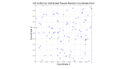
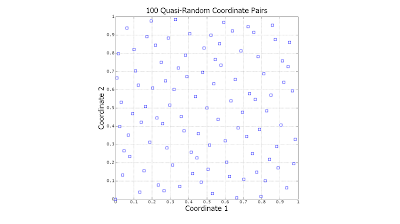
Notice the significant gaps left by the random data. There is nothing "wrong" with this: However undesirable, this is exactly how uniformly-distributed random data is expected to behave. In contrast, the quasi-random data is much more evenly distributed.
At this point, a question which might logically occur to the reader is, "Why not simply search on a regularly-spaced grid?" Grid searching is certainly a viable alternative, but requires that one know ahead of time precisely how many coordinates need to be generated. If the oil company in our example searches over a grid and discovers later that it has the budget for less or more tests than it originally planned, then the grid search will be sub-optimal. One very convenient property of quasi-random numbers is that however few or many are generated, they will (more-or-less) spread out as evenly as possible.
Clever as they are, most readers will be familiar with the pseudo-random number generators provided in base MATLAB, rand and randn. See, for instance the posts:
Dec-07-2006: Quick Tip Regarding rand and randn
Jan-13-2007: Revisiting rand (MATLAB 2007a)
Mar-23-2008: A Quick Introduction to Monte-Carlo and Quasi-Monte Carlo Integration
Quasi-random number generation is a recent addition to the MATLAB Statistics Toolbox (as of v6.2). The relevant functions are qrandstream, sobolset (Sobol generator) and haltonset (Halton generator). Other quasi-random number code can also be found for free via on-line searching (see the Nov-14-2006 post, Finding MATLAB Source Code And Tools). To research this subject further, look for material on "low discrepancy" sequences (the more technical name for quasi-random numbers).
Sunday, March 16, 2008
MATLAB 2008a Released
While not on disk yet, MATLAB release 2008a (MATLAB 7.6) is available for download from the MathWorks for licensed users. This release brings news on several fronts:
The Statistics Toolbox has seen a number of interesting additions, including: quasirandom number generators and (sequential) feature selection and cross-validation for modeling functions.
Another change which may be of interest to readers of this log is the upgrade of the Distributed Computing Toolbox, now named the Parallel Computing Toolbox. This Toolbox permits (with slight restructuring of MATLAB code) the distribution of the computational workload over multiple processors or processor cores. With more and more multi-core computers being sold every month, this offers the opportunity to greatly accelerate MATLAB code execution (think in terms of multiples of performance, not mere percentages!) to a very broad audience. Code which can be parallelized will run nearly twice as fast on a dual-core machine, and nearly four times as fast on a quad-core machine.
On a non-technical note, MATLAB has finally moved beyond software keys to on-line authentication for software installation. Is this good or bad? Both, I suppose. I'm sure that the MathWorks experiences its share of software piracy, so this move is understandable. It's also worth mentioning that MATLAB licensing is still very casual, with "one user" licensing still permitting installation on multiple machines (such as work and home), with the understanding that only one licensed person will use the software at a time.
Saturday, March 01, 2008
An Update on the Status of this Web Log
Four calendar months have elapsed with no technical update to this Web log. Judging by visitation statistics, though, this log is more popular than ever, ironically enough.
I do very much appreciate the kind words which appear from readers in the comments sections and in private communication. This Web log will continue to be updated, though for personal reasons, perhaps less frequently.
I do very much appreciate the kind words which appear from readers in the comments sections and in private communication. This Web log will continue to be updated, though for personal reasons, perhaps less frequently.
Subscribe to:
Comments (Atom)