Probability: A Halloween Puzzle

Introduction

Though Halloween is months away, I found the following interesting and thought readers might enjoy examining my solution.

Recently, I was given the following probability question to answer:

Halloween Probability Puzzler

The number of trick-or-treaters knocking on my door in any five minute interval between 6 and 8pm on Halloween night is distributed as a Poisson with a mean of 5 (ignoring time effects). The number of pieces of candy taken by each child, in addition to the expected one piece per child, is distributed as a Poisson with a mean of 1. What is the minimum number of pieces of candy that I should have on hand so that I have only a 5% probability of running out?

I am not aware of the author of this puzzle nor its origin. If anyone cares to identify either, I'd be glad to give credit where it's due.


Interpretation

I interpret the phrase "ignoring time effects", above, to mean that there is no correlation among arrivals over time; in other words, the count of trick-or-treater arrivals during any five minute interval is statistically independent of the counts in the other intervals.

So, the described model of trick-or-treater behaviors is that they arrive in random numbers during each time interval, and each take a single piece of candy plus a random amount more. The problem, then, becomes finding the 95th percentile of the distribution of candy taken during the entire evening, since that's the amount beyond which we'd run out of candy 5% of the time.


Solution Idea 1 (A Dead End)

The most direct method of solving this problem, accounting for all possible outcomes, seemed hopelessly complex to me. Trying to match each possible number of pieces of candy taken over so many arrivals over so many intervals results in an astronomical number of combinations. Suspecting that someone with more expertise in combinatorics than myself might see a way through that mess, I quickly gave up on that idea and fell back to something I know better: the computer (leading to solution idea 2... ).


Solution Idea 2

The next thing which occurred to me was Monte Carlo simulation, which is way of solving problems by approximating probability distributions using many random samples from those distributions. Sometimes very many samples are required, but contemporary computer hardware easily accommodates this need (at least for this problem). With a bit of code, I could approximate the various distributions in this problem and their interactions and have plenty of candy come October 31.

While Monte Carlo simulation and its variants are used to solve very complex real-world problems, the basic idea is very simple: Draw samples from the indicated distributions, have them interact as they do in real life, and accumulate the results. Using the poissrnd() function provided in the MATLAB Statistics Toolbox, that is exactly what I did (apologies for the dreadful formatting):

% HalloweenPuzzler
% Program to solve the Halloween Probability Puzzler by the Monte Carlo method
% by Will Dwinnell
%
% Note: Requires the poissrnd() and prctile() functions from the Statistics Toolbox
%
% Last modified: Apr-02-2014


% Parameter
B = 4e5;   % How many times should we run the nightly simulation?

% Initialize
S = zeros(B,1);  % Vector of nightly simulation totals


% Loop over simulated Halloween evenings
for i = 1:B
  % Loop over 5-minute time intervals for this night
  for j = 1:24
    % Determine number of arrivals tonight
    Arrivals = poissrnd(5);
   
    % Are there any?
    if  (Arrivals > 0)
      % ...yes, so process them.
     
      % Loop over tonight's trick-or-treaters
      for k = 1:Arrivals
        % Add this trick-or-treater's candy to the total
        S(i) = S(i) + 1 + poissrnd(1);
      end
    end
  end
end

% Determine the 95th percentile of our simulated nightly totals for the answer
disp(['You need ' int2str(prctile(S,95)) ' pieces of candy.'])


% Graph the distribution of nightly totals
figure
hist(S,50)
grid on
title({'Halloween Probability Puzzler: Monte Carlo Solution',[int2str(B) ' Replicates']})
xlabel('Candy (pieces/night)')
ylabel('Frequency')




% EOF


Fair warning: This program takes a long time to run (hours, if run on a slow machine).

Hopefully the function of this simulation is adequately explained in the comments. To simulate a single Halloween night, the program loops over all time periods (there are 24 intervals, each 5-minutes long, between 6:00 and 8:00), then all arrivals (if any) within each time period. Inside the innermost loop, the number of pieces of candy taken by the given trick-or-treater is generated. The outermost loop governs the multiple executions of the nightly simulation.

The poissrnd() function generates random values from the Poisson distribution (which are always integers, in case you're fuzzy on the Poisson distribution). Its lone parameter is the mean of the Poisson distribution in question. A graph is generated at the end, displaying the simulated distribution for an entire night.



Important Caveat

Recall my mentioning that Monte Carlo is an approximate method, several paragraphs above. The more runs through this process, the closer it mimics the behavior of the probability distributions. My first run used 1e5 (one hundred thousand) runs, and I qualified my response to the person who gave me this puzzle that my answer, 282, was quite possibly off from the correct one "by a piece of candy or two". Indeed, I was off by one piece. Notice that the program listed above now employs 4e5 (four hundred thousand) runs, which yielded the exactly correct answer, 281, the first time I ran it.

A Quick Introduction to Monte-Carlo and Quasi-Monte Carlo Integration

In a surprising range of circumstances, it is necessary to calculate the area or volume of a region. When the region is a simple shape, such as a rectangle or triangle, and its exact dimensions are known, this is easily accomplished through standard geometric formulas. Often in practice, however, the region's shape is irregular and perhaps of very high dimension. Some regions used in financial net present value calculations, for instance, may lie in spaces defined by hundreds of dimensions!

One method for estimating the areas of such regions is Monte Carlo integration. This is a conceptually simple, but very effective solution for some difficult problems. The basic idea is to sample over a region of known area, checking whether sampled points are within the region of interest or not. The proportion of sampled points found to lie within the region of interest multiplied by the (already known) area of the sampled region is an approximation of the area occupied by the region of interest. A related technique, Quasi-Monte Carlo integration, utilizes quasirandom ("low discrepancy") numbers in place of random ones.

An Example

To illustrate Monte Carlo integration, consider a problem with a known analytical solution: calculating the area of a circle. Suppose our circle lies within the unit square, ranging from 0.0 to 1.0 on both dimensions. This circle's center is at (0.5,0.5) and has a radius of 0.5. By the well-known formula, area of a circle = pi * radius squared, this circle has an area of:


>> pi * (0.5 ^ 2)

ans =

0.7854


Using MATLAB to approximate this measurement using Monte Carlo, we have:


>> n = 1e5; % Set number of samples to draw
>> rand('twister',9949902); % Initialize pseudorandom number generator
>> A = rand(n,2); % Draw indicated number of 2-dimensional coordinates in unit square
>> AA = sqrt(sum((A' - 0.5) .^ 2))' <= 0.5; % Determine whether samples are within circular region of interest
>> mean(AA) % Estimate area of the circle via the Monte Carlo method

ans =

0.7874


So, after one hundred thousand samples we are off by a small amount. Note that in this case, the area of the total sampled region is 1.0, so there's no need to divide. Let's see how well the Quasi-Monte Carlo technique performs:


>> n = 1e5; % Set number of samples to draw
>> HSet = haltonset(2); % Set up the Halton quasirandom process for 2-dimensional samples
>> B = net(HSet,n); % Draw indicated number of samples using quasirandom numbers
>> BB = sqrt(sum((B' - 0.5) .^ 2))' <= 0.5; % Determine whether samples are within circular region of interest
>> mean(BB) % Estimate area of the circle via the quasi-Monte Carlo method

ans =

0.7853


In this instance (and this will be true for many problems), quasirandom numbers have converged faster.

See also the Mar-19-2008 posting, Quasi-Random Numbers. As mentioned in that post, coordinates of a regular grid could be substituted for the random or quasirandom numbers, but this requires knowing in advance how many samples are to be drawn, and does not allow arbitrary amounts of further sampling to be used to improve the approximation.

Naturally, one would never bother with all of this to calculate the area of a circle, given the availability of convenient formula, but Monte Carlo can be used for regions of arbitrary, possibly highly irregular- even disjoint- regions. As with the bootstrap, simulated annealing and genetic algorithms, this method is made possible by the fact that modern computers provide tremendous amounts of rapid, accurate computation at extremely low cost.

Further Reading

For a good overview of the Monte Carlo method, see:

Monte Carlo Method

Quasi-Random Numbers

Many computer users, whether MATLAB programmers or not, are familiar with random numbers. Strictly speaking, the "random" numbers most often encountered on computers are known as pseudo-random numbers. Pseudo-random numbers are not actually "random" at all, as they are deterministically generated in a completely repeatable fashion using one of a number of algorithms called pseudo-random number generators ("PRNG", if you want to impress your friends with lingo). Pseudo-random numbers are designed to mimic specific statistical distributions, most often the uniform distribution or, somewhat less commonly, the normal distribution.

The usefulness of random (or pseudo-random) numbers cannot be overestimated. They are used in computers for such different purposes as optimization, numerical integration, machine learning, simulation and scheduling. A common theme among these applications is the utilization of random numbers to cover or search a geometric space, most often accomplished via uniformly distributed random numbers. In such cases, sets of random numbers define the coordinates of single points in the searched space.

As a simplified example, think of a petroleum company searching for oil in a square plot of land. With no knowledge of where the oil may lie, and a limited budget for drilling holes, the company requires some method for selecting locations to test. Uniformly distributed random numbers could be used for this purpose, but they present a subtle deficiency, informally known as "clumping". Since each coordinate pair is drawn completely independently and the random numbers being used are uncorrelated with one another, there is the real possibility that test sites will be specified near existing test sites. One would imagine that new test sites within our square should be as far as possible from sites already tested. Whether existing sites are dry or not, testing very near them would seem to add little information.

Perhaps a better choice in such circumstances would be quasi-random numbers. Quasi-random numbers behave something like random numbers, but are generated as correlated vectors, so as to better obey the intended distribution, even in multiple dimensions. In our oil drilling problem, quasi-random numbers could be generated in pairs to form coordinates for drilling sites. Such coordinates would be less likely to fall near those already generated. Quasi-random numbers are known to converge to a solution faster than random ones in a variety of problems, such as numeric integration.

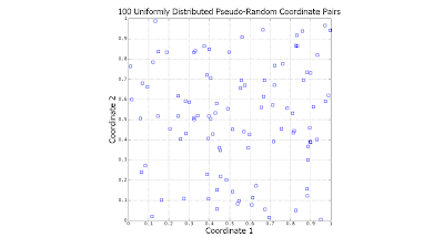
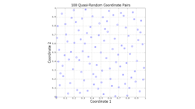
The following scatter plots illustrate the difference between the two (click to enlarge):





Notice the significant gaps left by the random data. There is nothing "wrong" with this: However undesirable, this is exactly how uniformly-distributed random data is expected to behave. In contrast, the quasi-random data is much more evenly distributed.

At this point, a question which might logically occur to the reader is, "Why not simply search on a regularly-spaced grid?" Grid searching is certainly a viable alternative, but requires that one know ahead of time precisely how many coordinates need to be generated. If the oil company in our example searches over a grid and discovers later that it has the budget for less or more tests than it originally planned, then the grid search will be sub-optimal. One very convenient property of quasi-random numbers is that however few or many are generated, they will (more-or-less) spread out as evenly as possible.

Clever as they are, most readers will be familiar with the pseudo-random number generators provided in base MATLAB, rand and randn. See, for instance the posts:

Dec-07-2006: Quick Tip Regarding rand and randn
Jan-13-2007: Revisiting rand (MATLAB 2007a)
Mar-23-2008: A Quick Introduction to Monte-Carlo and Quasi-Monte Carlo Integration

Quasi-random number generation is a recent addition to the MATLAB Statistics Toolbox (as of v6.2). The relevant functions are qrandstream, sobolset (Sobol generator) and haltonset (Halton generator). Other quasi-random number code can also be found for free via on-line searching (see the Nov-14-2006 post, Finding MATLAB Source Code And Tools). To research this subject further, look for material on "low discrepancy" sequences (the more technical name for quasi-random numbers).

Revisiting rand (MATLAB 2007a)

Pseudo-random number generators (PRNG) are frequently used in statistical and machine learning methods for things like train/test selection and solution initialization. (See an interesting discussion of this in the Nov-22-2006 posting, Explicit Randomization in Learning algorithms, on the Machine Learning (Theory) log.) Hence, it is important to understand the operation of the pseudo-random number generator employed in one's code.

I've just gotten word that MATLAB's built-in rand function will be changing (as of MATLAB 2007a) to use the Mersenne Twister method of generating numbers be default. Note that use of 'state' or 'seed' will change to a generator other than the default. Probably the most important impact at a practical level is that code not specifying another generator (not using 'state' or 'seed') will now generate different values.

Note, too, that if the randperm function continues to follow rand's lead (randperm was initialized by initializing rand in the past), then it will also produce different values than in previous releases if rand is not initialized.

I have no word on whether this affects randn or not.

MATLAB programming suggestion: Always initialize the random number functions before calling them. Repeatable results make testing code much easier.

See my post of Dec-07-2006, Quick Tip Regarding rand and randn for more information on rand and randn.

Also see the Mar-19-2008 post, Quasi-Random Numbers.

Also in 2007a, "divide-by-zero" and "log-of-zero" warning messages will be turned off by default.