In my work, I have frequently needed to fit curves to data. Curve-fitting is a broad and surprisingly subtle subject. The two most common types of single-input curve-fitting are simple (linear and non-linear) regression and splines.
Regressions involve the discovery of optimal coefficients for some functional form, which maps the input variable to the output variable. Regressions provide a number of advantages, but these are generally qualified advantages:
Regression Characteristics
1. Common functions (linear, logistic, exponential) are well-studied and widely available. More exotic or arbitrary functions are harder to find software for.
2. Regressions provide optimal fit to data, assuming that one wants a least-squares fit. Some software, notably the MATLAB Curve Fitting Toolbox, will provide other, less common fits, such as mean absolute error (L-1) and robust fits.
3. Regressions are the safest bet for extrapolation. Extrapolation is a hazardous endeavor, but well-behaved regression functions generate the most sensible guess in "the far, unlit unknown".
4. Complex regression curves, such as high-order polynomials, can be ill-behaved, especially at the extremes of the data range. While there are methods of combatting such problems (such as fitting at the Chebyshev points), these are not widely available in commercial software.
Splines, which are especially popular in engineering, are connected series of simple curves, most often low-order polynomials. The advantage of splines is that they are extremely flexible. Complex curves require complex regression functions, but splines can handle very complicated shapes simply by connecting several simple curves. Splines may pass directly through data points, or between them. To maintain continuity, these simple curves must come together at points called knots. Like regressions, splines have their advantages:
Spline Characteristics
1. Splines are extremely flexible, but number and placement of knots must be chosen.
2. Technically, most splines are undefined outside the range of the knots.
3. Most commercial software is oriented toward locating a spline through a small number of given data points. "Fitting" through a large number of data points is not commonly available.
Additionally, base MATLAB directly supports the construction and evaluation of splines.
GASplineFit
Wanting to free myself from having to select the right regression function every time I needed to fit a curve, I decided to turn to splines for my curve-fitting needs. The problem, as mentioned above, is that almost all spline routines and canned software are very low-level, "fitting" (if it can be called that) splines by stringing them through a very small number of selected points. My solution, GASplineFit.m, builds on the built-in MATLAB spline routines, and will generate splines which optimize any error function handled by my SampleError routine (see my posting of Jan-05-2007, Model Performance Measurement). Note: GASplineFit requires subroutine LogRand.m.
With GASplineFit, the user supplies:
1. An input variable
2. An output variable
3. The input values of the knots (I often just use linspace for these)
4. The spline type (such as 'pchip' or 'spline': see MATLAB's spline routines)
5. A selected performance measure ('MSE', 'L-1', etc.).
There are two additional parameters, which control the genetic algorithm which performs the fitting. I usually don't change these from 250 and 80. For better but slower fitting, turn these parameters up. For faster but cruder fitting, turn them down. See help GASplineFit for details.
Essentially, the software is sliding the spline knots up and down, trying to get this best fit. The routine returns:
1. The fitted spline as a MATLAB piecewise polynomial (see: help ppval)
2. The knot output values
3. The assessed error
Notice one very nice feature of this routine: that it will fit probability curves directly to 0/1 data. Very often, the statistician is faced with a large collection of examples, which involve a dummy variable indicating membership in a class of interest, and an explanatory variable. To smooth the data and approximate the probability of class membership, common practice is to bin the explanatory variable, and assess the mean for each bin. Fancier methods will fit a curve to these binned values, which isn't very smooth or use a kernel regression, which is smooth but typically difficult to encapsulate as code without taking the entire data set along for the ride. GASplineFit solves all of these problems. The genetic algorithm which is its engine doesn't care about the fact that our data may be only zeros and ones: it only cares about optimizing the performance function.
help GASplineFit explains the specifics of this routine, and provides an example of its use. MATLAB programmers beginning with genetic algorithms may be interested in examining the code, which uses an elitist genetic algorithm.
Showing posts with label spline. Show all posts
Showing posts with label spline. Show all posts
Friday, January 19, 2007


Thursday, November 16, 2006
Fuzzy Logic In MATLAB Part 1
Fuzzy logic is a capable and often misunderstood analytical tool. A basic grasp of this technology may be gained from any of the following introductions to fuzzy logic:
Putting Fuzzy Logic to Work (PDF), PC AI magazine, by Dwinnell
Fuzzy Math, Part 1, The Theory, by Luka Crnkovic-Dodig
Fuzzy Logic Introduction (PDF), by Martin Hellmann
Fuzzy Logic Overview (HTML)
comp.ai.fuzzy FAQ: Fuzzy Logic and Fuzzy Expert Systems
Fuzzy Logic for "Just Plain Folks" (HTML), by Thomas Sowell
As a rule, in the interest of portability and transparency, I try to build as much of my code as possible in base MATLAB, and resort to using toolboxes and such only when neccessary. Fortunately, fuzzy logic is exceedingly easy to implement in the base MATLAB product.
Generation of fuzzy set memberships can be accomplished using the base MATLAB functions interp1 and pchip. Piecewise linear (most commonly: triangular and trapezoidal) fuzzy memberships can be calculated using the 'linear' method in interp1. Below is an example of a triangular fuzzy memebership function, defined over the Temperature domain (click the graph to enlarge):
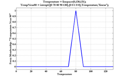
The domain variable and shape parameters (domain vector followed by membership vector) control the form of the curve. Trapezoids are constructed by adding another element to each shape vector, like this:
Temperature = linspace(0,130,131);
Temp80ish = interp1([0 70 78 82 90 130],[0 0 1 1 0 0],Temperature,'linear');
Fuzzy membership functions with smoother transitions are possible by using the pchip function. The following depicts a bell-shaped membership function (as usual, click the graph to enlarge):
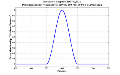
Of course, one is not limited to peaked or plateau-shaped fuzzy membership functions. The various interpolation and spline functions in MATLAB permit whatever irregular and arbitrary shapes may be called for.
In Part 2, I will build a small fuzzy rule base in MATLAB.
Further Reading
Print:
An excellent practical reference:
The Fuzzy Systems Handbook (Second Edition), by Cox (ISBN: 0121944557)
Putting Fuzzy Logic to Work (PDF), PC AI magazine, by Dwinnell
Fuzzy Math, Part 1, The Theory, by Luka Crnkovic-Dodig
Fuzzy Logic Introduction (PDF), by Martin Hellmann
Fuzzy Logic Overview (HTML)
comp.ai.fuzzy FAQ: Fuzzy Logic and Fuzzy Expert Systems
Fuzzy Logic for "Just Plain Folks" (HTML), by Thomas Sowell
As a rule, in the interest of portability and transparency, I try to build as much of my code as possible in base MATLAB, and resort to using toolboxes and such only when neccessary. Fortunately, fuzzy logic is exceedingly easy to implement in the base MATLAB product.
Generation of fuzzy set memberships can be accomplished using the base MATLAB functions interp1 and pchip. Piecewise linear (most commonly: triangular and trapezoidal) fuzzy memberships can be calculated using the 'linear' method in interp1. Below is an example of a triangular fuzzy memebership function, defined over the Temperature domain (click the graph to enlarge):

The domain variable and shape parameters (domain vector followed by membership vector) control the form of the curve. Trapezoids are constructed by adding another element to each shape vector, like this:
Temperature = linspace(0,130,131);
Temp80ish = interp1([0 70 78 82 90 130],[0 0 1 1 0 0],Temperature,'linear');
Fuzzy membership functions with smoother transitions are possible by using the pchip function. The following depicts a bell-shaped membership function (as usual, click the graph to enlarge):
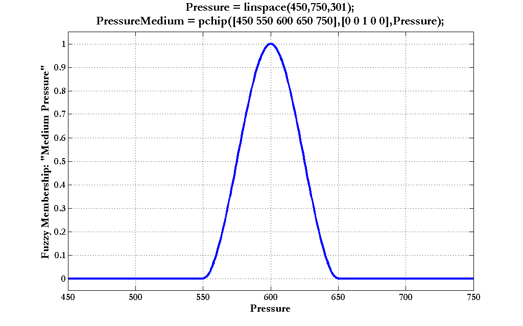
Of course, one is not limited to peaked or plateau-shaped fuzzy membership functions. The various interpolation and spline functions in MATLAB permit whatever irregular and arbitrary shapes may be called for.
In Part 2, I will build a small fuzzy rule base in MATLAB.
Further Reading
Print:
An excellent practical reference:
The Fuzzy Systems Handbook (Second Edition), by Cox (ISBN: 0121944557)
Subscribe to:
Posts (Atom)